In the previous article we have seen that there are many possibilities for the structure of an alloy. The properties of a material depend on the type, number, amount, and form of the phases present, and can be changed by altering these quantities. In order to make these changes, it is essential to know the conditions under which these quantities exist and the conditions under which a change in phase will occur.
The best method to record the data related to phase changes in alloy systems is in the form of phase diagrams, also known as equilibrium diagrams or constitutional diagrams.
In order to specify completely the state of a system in equilibrium, it is necessary to specify three independent variables. These variables, which are externally controllable, are temperature, pressure and composition. With pressure assumed to be constant at atmospheric value, the equilibrium diagram indicates the structural changes due to variation of temperature and composition.
Phase diagram show the phase relationships under equilibrium conditions, that is, under conditions in which there will be no change with time. Equilibrium conditions may be approached by extremely slow heating and cooling, so that if a phase change is to occur, sufficient time is allowed.
Thus, the phase diagram is simply a map showing the structure of phases present as the temperature and overall composition of the alloy are varied. A binary phase diagram shows the phases formed in differing mixtures of two components over a range of temperatures. When an alloy has more than two components, a different type of phase diagram must be used, such as a ternary diagram for three phase alloys and so on.
For mechanical engineers, study of binary phase diagrams classified as under will be adequate to gain knowledge on basic principles of phase diagrams.
1. Components completely soluble in the liquid state and
a. Completely soluble in the solid state (Type I)
b. Insoluble in the solid state: the eutectic reaction (Type II)
c. Partly soluble in the solid state: the eutectic reaction (Type III)
d. Formation of a congruent-melting intermediate phase (Type IV)
e. The peritectic reaction (Type V)
2. Transformations in the solid state
a. Allotropic change
b. Order-disorder
c. The eutectoid reaction
d. The peritectoid reaction
Information about construction of a phase diagram and study of a phase diagram where components of the alloy are completely soluble in both the liquid and solid states (Type I) is given in this article. Information on the remaining types of phase diagrams will be covered in the next article titled Phase Diagrams (Part 2).
It may be noted that information about following two types of diagrams is not given in this article as the article is written for mechanical engineers.
1. Components partly soluble in the liquid state. The monotectic reaction and
2. Components insoluble in the liquid state and insoluble in the solid state.
Coordinates of Phase Diagram and Experimental Methods
Phase diagrams are usually plotted with temperature as the ordinate, and the alloy composition in weight percentage as the abscissa. Sometimes alloy composition is expressed in atomic percentage for certain type of scientific work as it is more convenient that way.
The data for the construction of equilibrium diagrams are determined experimentally by a variety of methods, the most common methods are as under.
Metallographic Methods
This method is applied by heating samples of an alloy to different temperatures, waiting for equilibrium to be established, and then quickly cooling to retain their high-temperature structure. The samples then examined microscopically. This method is difficult to apply to metals at high temperatures because the rapidly cooled samples do not always retain their high-temperature structure, and considerable skill is then required to interpret the observed microstructure correctly.
X-ray Diffraction Technique
This method is applied by measuring the lattice dimensions and indicating the appearance of a new phase either by the change in lattice dimension or by the appearance of a new crystal structure. This method is very precise and very useful in determining the changes in solid solubility with temperature.
Thermal Analysis
This is by far the most widely used experimental method. It relies on the information obtained from the cooling curves. In this method, alloys mixed at different compositions are melted and then the temperature of the mixture is measured at a certain time interval while cooling back to room temperature. This method seems to be best for determining the initial and final temperature of solidification. Phase changes occurring solely in the solid state generally involve only small heat changes, and other methods give more accurate results.
Two Metals Completely Soluble in the Liquid and Solid States (Type I)
Since the two metals are completely soluble in the solid state, the only type of solid phase formed will be a substitutional solid solution. The two metals will generally have the same type of crystal structure and differ in atomic radii by less than 8 percent.
Construction of Phase Diagram
The result of running a series of cooling curves for various combinations or alloys between metals A and B, varying in composition from 100 percent A & 0 percent B to 0 percent A & 100 percent B is shown in the diagram at LHS in the figure given below.
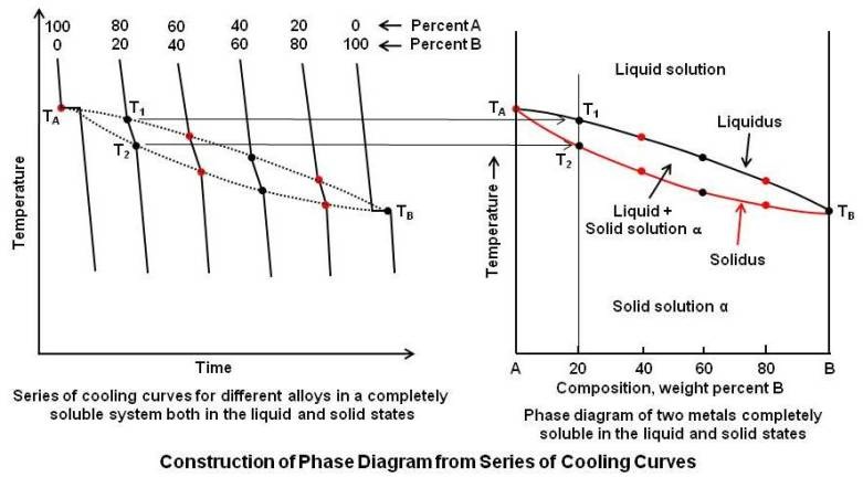
It may be noted that each cooling curve is a separate experiment starting from zero time. The cooling curves for the pure metals A and B show only a horizontal line because the beginning and end of solidification take place at a constant temperature. However, since intermediate compositions form a solid solution, these cooling curves shows two breaks or change in slope. For an alloy containing 80A and 20B, the first break is at temperature T1, which indicates the beginning of solidification, and the lower break at T2 indicates the end of solidification. All intermediate alloy compositions will show a similar type of cooling curve.
It is now possible to construct actual phase diagram by plotting temperature vs. composition. The appropriate points are taken from the series of cooling curves and plotted on the new diagram as shown by the diagram at RHS in the above figure.
Since the left axis represents the pure metal A, TA is plotted along this line. Similarly, TB is plotted. Since all intermediate compositions are percentages of A and B, for simplicity the percent sign is omitted. A vertical line representing the alloy 80A-20B is drawn, and T1 and T2 from cooling curve are plotted along this line. The same procedure is used for the other compositions.
The phase diagram consists of two points, two lines, and three areas. The two points TA and TB represent the freezing points of the two pure metals. The upper line, obtained by connecting the points showing the beginning of solidification, is called the liquidus; and the lower line, determined by connecting the points showing the end of solidification, is called the solidus line. The area above the liquidus line is a single-phase region, and any alloy in that region will consist of a homogeneous liquid solution. Similarly, the area below the solidus line is a single-phase region, and any alloy in this region will consist of a homogeneous solid solution. It is common practice, in labeling of equilibrium diagrams, to represent solid solution and sometimes intermediate alloys by Greek letters. In this case, it is labeled the solid solution alpha (α). Upper case letters A and B are used to represent the pure metals. Between the liquidus and solidus lines there exists a two-phase region. Any alloy in this region will consist of a mixture of a liquid solution and a solid solution.
Specification of temperature and composition of an alloy in a two-phase region indicates that the alloy consists of a mixture of two phases but does not give any information about the actual chemical composition and the relative amounts of the two phases that are present. They can be determined as under.
Chemical Composition of Phases
To determine the actual chemical composition of the phases of an alloy, draw a horizontal temperature line, called a tie line, to the boundaries of the field as shown in the figure given below.
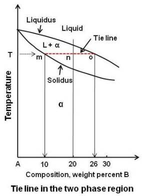
The points of intersection are dropped to the base line, and the composition is read directly.
In the above figure, consider the alloy composed of 80A-20B at the temperature T. The alloy is in a two-phase region. To find the composition, draw the tie line mo to the boundaries of the field. Point m, the intersection of tie line with the solidus line, when dropped to the base line, gives the composition of the phase that exists at that boundary. In this case, the phase is a solid solution of α of composition 90A-10B. Similarly, point o, when dropped to the base line, will give the composition of the other phase constituting the mixture, in this case the liquid solution of composition 74A-26B.
Relative Amounts of Each Phase (The Lever Rule)
To determine the relative amounts of the two phases, draw a vertical line representing the alloy and a horizontal temperature line to the boundaries of the field (tie line). The vertical line will divide the horizontal line into two parts whose lengths are inversely proportional to the amount of the phases present. This is also known as the Lever Rule. The point where the vertical line intersects the horizontal line may be considered as the fulcrum of a lever system. The relative lengths of the lever arms multiplied by the amounts of the phases present must balance.
In the above figure, the vertical line, representing the alloy 20B, divides the horizontal tie line into two parts, mn and no. If the entire length of the tie line mo is taken to represent 100 percent, or the total weight of the two phases present at temperature T, the lever rule may be expressed mathematically as:
Liquid (percent) = (mn / mo) x 100
Solid α (percent) = (no / mo) x 100
By inserting the numerical values, we get
Liquid (percent) = (10 / 16) x 100 = 62.5
Solid α (percent) = (6 / 16) x 100 = 37.5
The above may be summarized as; the alloy of composition 80A-20B at temperature T consists of a mixture of two phases. One is liquid solution of composition 74A-26B consisting 62.5 percent of all the material present and the other a solid solution of composition 90A-10B making up 37.5 percent of the material present.
Note that the right side of the tie line gives the proportion of the phase on the left (α phase in this example) and left side of the tie line gives the proportion of the phase to the right (liquid phase in this example).
Equilibrium Cooling of a Solid Solution Alloy
Phase changes that occur at various stages during equilibrium cooling of a solid solution alloy from liquid state to solid state are explained below. The process is explained with reference to the phase diagram given below by showing what happens in a particular alloy 70A-30B as it is cooled from liquid state to solid state.
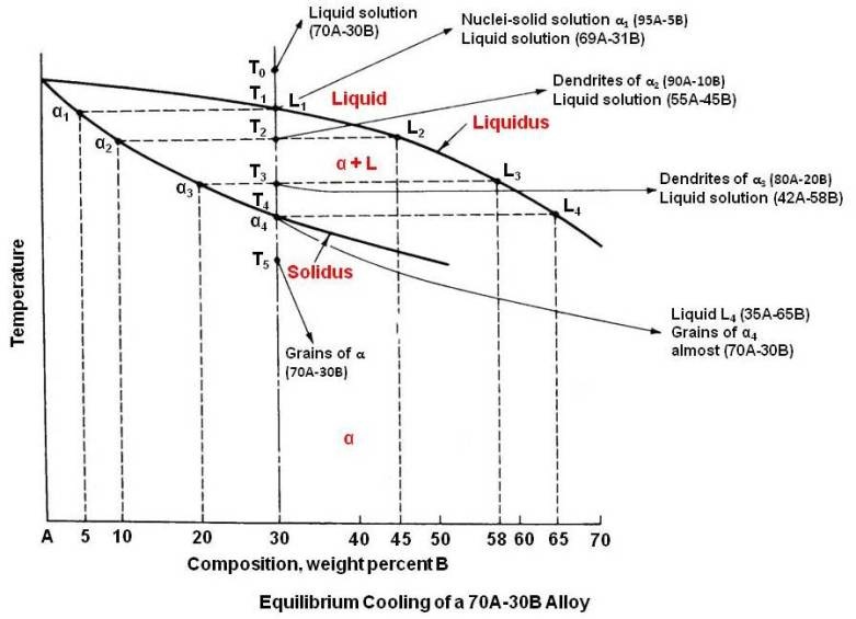
The alloy at temperature T0 is a homogeneous single-phase liquid solution and remains so until temperature T1 is reached. Since T1 is on the liquidus line, freezing/solidification now begins. The first nuclei of solid solution to form, α1, will be very rich in the higher-melting-point metal A and will be composed of 95A-5B. Since the solid solution in forming takes material very rich in A from the liquid, the liquid must get richer in B. In view of this, just after the solidification, the composition of the liquid is approximated as 69A-31B.
When the lower temperature T2 is reached, the liquid composition is at L2. The only solid solution in equilibrium with L2 and therefore the only solid solution forming at T2 is α2. It can be seen from the diagram that α2 is composed of 10B. Hence, as the temperature is decreased, not only does the liquid composition become reach in B but also the solid solution. At T2, crystals of α2 are formed surrounding the α1 composition cores (primary dendrites α1) and also separate dendrites of α2 as shown in the figure given below.
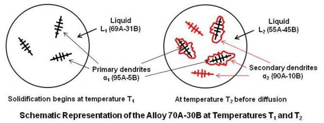
In order for the equilibrium to be established at T2, the entire solid phase must be a composition α2. This requires diffusion of B atoms to the A rich core not only from the solid just formed but also from the liquid. This is possible only if the cooling is extremely slow so that diffusion may keep pace with crystal growth.
At any temperature, the relative amounts of the liquid and solid solution may be determined by Lever Rule.
As the temperature falls, the solid solution continues to grow at the expense of the liquid. At T3, the solid solution will make up approximately three-fourths of all the material present.
Finally, the solidus line is reached at T4 and the last liquid L4, very rich in B, solidifies primarily at the grain boundaries. However, diffusion will take place and all the solid solution will be of uniform composition α (70A-30B), which is the overall composition of the alloy.
Diffusion
The movement of atoms in the solid state, called diffusion is an important phenomenon. Through the mechanism of diffusion under slow cooling the dendritic structure disappears and the grains become homogeneous.
Diffusion is essentially statistical in nature, resulting from many random movements of individual atoms. While the path of an individual atom may be zigzag and unpredictable, when large number of atoms makes such movements they can produce a systematic flow. There are three methods by which diffusion in substitutional solid solutions may take place. They are the vacancy mechanism, interstitial mechanism and atom interchange mechanism as shown below.
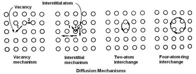
It has been found that the use of vacancies is the primary method of diffusion. The rate of diffusion is much greater in a rapidly cooled alloy than in the same alloy slow-cooled. The difference is due to the larger number of vacancies retained in the alloy by fast cooling. The rate of diffusion of one metal in another is a function of many variables, however the most important is temperature.
Nonequilibrium Cooling
In actual practice it is extremely difficult to cool under equilibrium conditions. Since diffusion in the solid state takes place at very slow rate, it is expected that with ordinary cooling rates there will be some difference in the conditions as indicated by the equilibrium diagram.
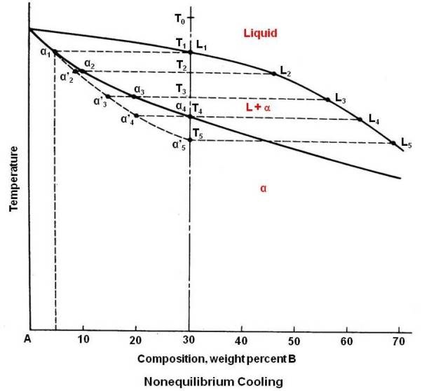
Diagram for Nonequilibrium cooling condition is given in the above figure. Solidification starts at T1 forming a solid solution of composition α1. At T2 the liquid is at L2 and the solid solution now forming is of composition α2. Since the diffusion is too slow to keep pace with crystal growth, not enough time will be allowed to achieve uniformity in the solid, and the average composition will be between α1 and α2 say α’2. As the temperature drops, the average composition of solid solution will depart still further from equilibrium conditions. It seems that the composition of the solid solution is following the nonequilibrium solidus line α1 to α’5 shown dotted in the above figure. The liquid, on the other hand, has essentially the composition given by the liquidus line, since diffusion is relatively rapid in liquid. At T3, the average solid solution will be of composition α’3 instead of α3. Under equilibrium cooling, solidification should be completed at T4, however, since the average composition of solid solution of α’4 has not reached the composition of the alloy, some liquid must still remain. Application of Lever Rule at T4 gives,
L4 (percent) = (α’4T4 / α’4L4) x 100 ≈ 25 percent
Solidification will therefore continue until T5 is reached. At this temperature the composition of the solid solution α’5 coincides with the alloy composition, and solidification is complete. The last liquid to solidify, L5, is richer in B than the last liquid to solidify under equilibrium conditions. Thus it is apparent from the study that the more rapidly the alloy is cooled the greater will be the composition range in the solidified alloy.
The final solid consists of a cored structure with a higher-melting central portion surrounded by the lower-melting, last-to-solidify shell. Thus as crystal grows, there will be a difference in chemical composition from the center to the outside of the grain. The above condition is referred to as coring or dendritic segregation.
Homogenization
Cored structures are most common in as-cast metals. The last solid formed along the grain boundaries and in the interdendritic spaces is very in the lower-melting-point metal. Depending upon the properties of this lower-melting-point metal, the grain boundaries may act as a place of weakness. It will result in a serious lack of uniformity in mechanical and physical properties and, in some cases, increased susceptibility to intergranular corrosion because of preferential attack by a corrosive medium. Therefore, for some applications, a cored structure is objectionable.
There are two ways to solve the coring problem. One is to prevent its formation by slow freezing from the liquid state, but this result in large grain size and requires a very long time. The other industrially preferred method is of homogenization of the cored structure by diffusion in the solid state.
At room temperature, for most metals, the diffusion rate is very slow, but if the alloy is reheated to a temperature below the solidus line, diffusion will be more rapid and homogenization will occur in a relatively short time. However, extreme care must be exercised in this treatment not to cross the solidus line; otherwise liquidation of grain boundaries will occur, damaging the shape and physical properties of the casting.
Properties of Solid Solution Alloys
In general, in an alloy system, most of the property changes are caused by distortion of the crystal lattice of the solvent metal by addition of the solute metal.
The effect of composition on some physical and mechanical properties of annealed alloys in the copper-nickel system is given below.
| Composition of Nickel | Tensile Strength, psi | Elongation, % in 2 in. | Electrical Resistivity, Microhms / Cm3 |
|---|---|---|---|
| 0 | 30000 | 53 | 1.7 |
| 10 | 35000 | 47 | 14 |
| 20 | 39000 | 43 | 27 |
| 30 | 44000 | 40 | 38 |
| 40 | 48000 | 39 | 46 |
| 50 | 50000 | 41 | 51 |
| 60 | 53000 | 41 | 50 |
| 70 | 53000 | 42 | 40 |
| 80 | 50000 | 43 | 30 |
| 90 | 48000 | 45 | 19 |
| 100 | 43000 | 48 | 6.8 |
Electrical resistivity depends on distortion of the lattice structure. Since the distortion increases with the amount of solute metal added, and since either metal can be considered as the solvent, the maximum electrical resistivity should occur in the center of the composition range. This is verified by the values given in the table. As copper is added to nickel, the strength of alloy increases, and nickel is added to copper, the strength of that alloy also increases. Therefore, between pure copper and pure nickel there must be an alloy which shows the maximum strength. It turns out to be at approximately two-thirds nickel and one-third copper. This is very useful commercial alloy known as Monel. It shows good strength and good ductility along with high corrosion resistance. The same behavior is also true of hardness in that there will be an alloy that shows the maximum hardness.
Variations of Type I
Every alloy in Type I system has a melting point between the melting points of A and B. It is possible to have a system in which the liquidus and solidus lines go through a minimum or a maximum as shown in the figure given below.
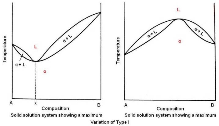
The alloy composition x in above figure behaves just like a pure metal. There is no difference in the liquid and solid composition. It begins and ends solidification at a constant temperature with no change in composition, and its cooling curve will show a horizontal line. Such alloys are known as congruent-melting alloys. Because alloy x has the lowest melting point in the series, and the equilibrium diagram resembles the eutectic type to be discussed in the next article. It is sometimes known as pseudoeutectic alloy. Example of alloy system that shows a minimum is Cu-Au.
Those showing a maximum temperature are rare and there are no known metallic systems of this type.
